How much survey is enough—and whose uncertainty matters?

This notebook is a 15-minute demonstration for a mixed audience at the Johns Hopkins International Vaccine Access Center (IVAC). It compares serosurvey designs using financial cost, overall estimation accuracy and accuracy for an underserved group. All populations, prevalences, prices and preference weights are hypothetical.

Open the executed Jupyter notebook to read the narrative, code, tables and saved figures. The accompanying Python script contains the simulator and plotting helpers and regenerates these figures. Use both files from a checkout; the notebook imports the companion module. The notebook addresses the presentation audience directly. Setup commands, export instructions and the suggested running order are collected in this guide.

Run or present the notebook

From the repository root:

uv run --extra notebook jupyter lab examples/serosurvey_study.ipynb

Choose the environment's Python kernel, then restart it and run all cells. The notebook extra supplies JupyterLab, nbconvert, pandas, matplotlib and Pareto analysis without requiring the other optional modeling backends. Installation needs network access; the executed example uses only local code and synthetic data. Run from a checkout of main: the notebook uses the preference API added after the 0.3.0 release.

Clean notebook executions took about six to eight seconds on the development machine, including kernel startup and rendering. The companion script took about two seconds for 19,800 evaluations and four figures. These measurements exclude dependency installation; check your presentation machine before the talk.

Saved notebook outputs provide a fallback without running code. Export them to HTML for an additional presentation copy:

uv run --extra notebook jupyter nbconvert --to html examples/serosurvey_study.ipynb

To omit the collapsed setup code from a presentation copy while keeping the analysis code visible:

uv run --extra notebook jupyter nbconvert --to html \
  --TagRemovePreprocessor.enabled=True \
  --TagRemovePreprocessor.remove_input_tags='["hide-input"]' \
  examples/serosurvey_study.ipynb

To verify execution in a fresh kernel without modifying the saved notebook:

uv run --extra notebook jupyter nbconvert --execute --to notebook \
  --ExecutePreprocessor.timeout=60 --output serosurvey_executed.ipynb \
  --output-dir /tmp examples/serosurvey_study.ipynb

The decision

IVAC's SISS project examined the design and use of serological surveillance. The serosurvey costing study by Carcelen, Patenaude, Moss and colleagues provides a concrete link between epidemiology and economic evaluation. Its study-, cluster- and participant-level cost structure motivates this example; we do not reproduce its study or use its historical prices.

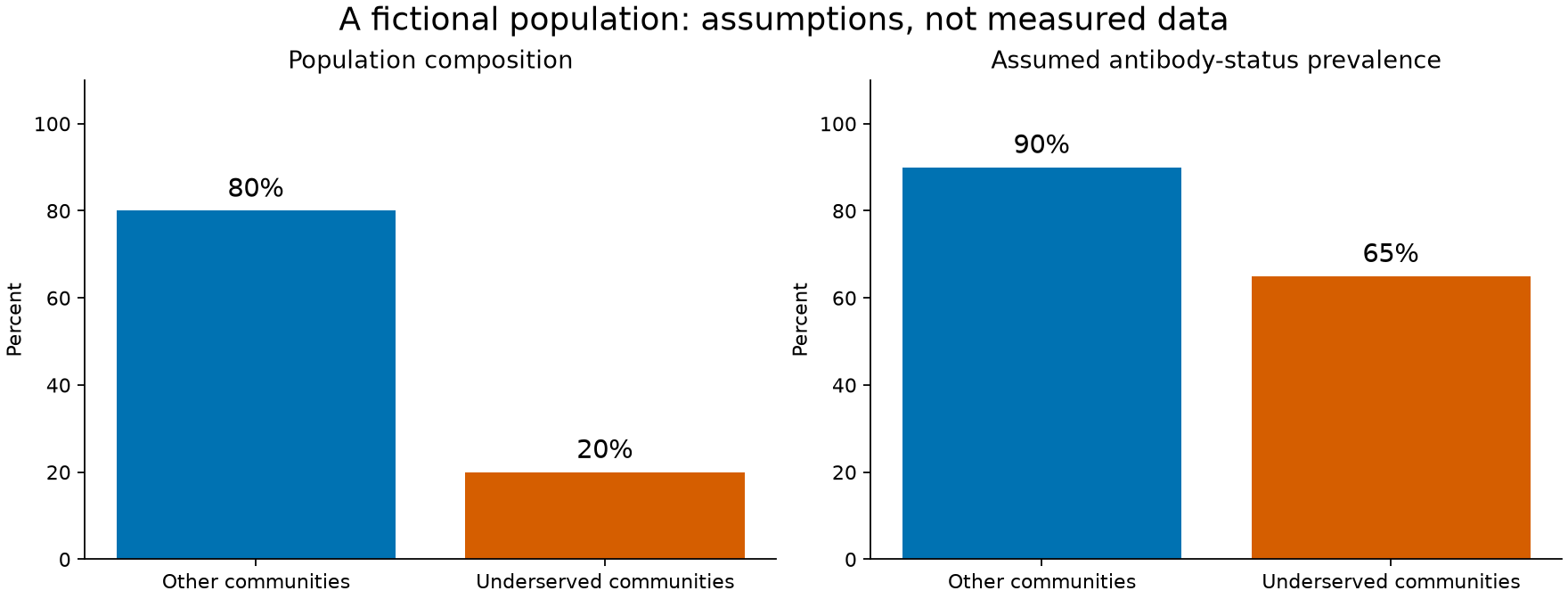
The fictional population consists of an 80% group and a 20% underserved group, with antibody-status prevalences of 90% and 65% respectively. These are assumed model inputs, not measured data or protection thresholds.

Compare 18 designs:

Factor	Levels
Participants	300, 600, 1,200
Communities	10, 20, 40
Allocation	Proportional 80:20, or oversampling 50:50

Allocation applies to both participants and communities. Within each group, participants are distributed as evenly as possible, keeping exact totals. Independent community probabilities follow a Beta distribution centered on the group mean, with illustrative within-community correlation 0.06; participant counts then follow a binomial model. The estimand is the fixed group mean, not the realized mean in the sampled communities.

The overall prevalence estimator uses population weights of 80:20 for both allocation strategies. Oversampling does not change the population composition. Financial cost is fixed setup plus community visit costs plus participant costs. Average per-community and per-participant costs are not added together as if they were independent marginal costs.

Run, aggregate and refine

The notebook visibly constructs a Study with two grid Phases: 100 simulated surveys per design, followed by 1,000 per design with an independent phase seed. Both phases evaluate all 18 designs. Refinement increases simulation replication, not the number of participants per survey. The refined estimates replace the screening estimates; the two phases are not pooled.

Each scorer call returns financial cost and absolute prevalence errors in percentage points. aggregate_replicates() averages those errors, producing mean absolute error (MAE), and retains their Monte Carlo variation. Averaging signed errors before taking their absolute value would measure something different.

Inspect feasible alternatives

A Constraint imposes an illustrative $40,000 financial budget. The Pareto set minimizes cost, overall MAE and underserved-group MAE simultaneously. Subgroup error is a narrow measure of information equity, not a comprehensive measure of equity in health outcomes.

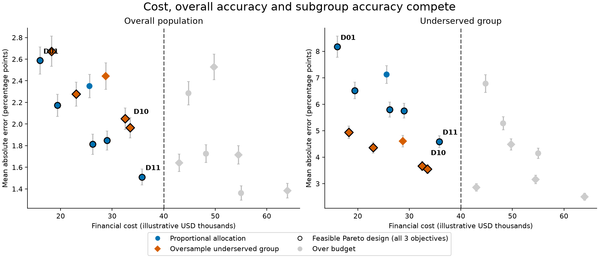
Gray designs exceed the budget. Outlines show the feasible Pareto set computed using all three objectives; the two panels are projections, not independently computed two-objective fronts. Design labels identify the preference winners. Vertical bars are approximately two Monte Carlo standard errors of estimated MAE. They express simulation precision under this model, not uncertainty in a real survey's prevalence or the model assumptions. They are marginal bars, not simultaneous post-selection confidence guarantees.

Change priorities without rerunning simulations

The notebook passes the raw results to preference_sweep() with three explicit preference vectors and normalization="reference". Fixed reference ranges are $0–70,000, 0–4 percentage points overall MAE, and 0–10 percentage points subgroup MAE. These anchors scale preferences; they are not feasibility thresholds and do not clip values. Scenario weights are hypothetical, not elicited stakeholder values.

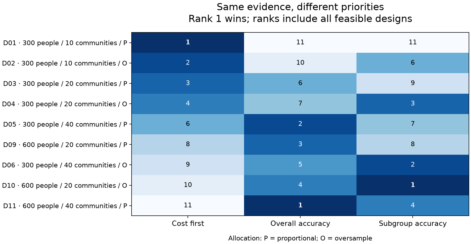
Rank 1 wins within a scenario. The displayed rows are feasible Pareto designs, but ranks include all feasible designs. Choices depend on point estimates and can change with further simulation or different assumptions. Any reported selection fraction describes the supplied preference scenarios, not a probability that a design is best.

For a short live interaction, change the budget to $30,000 in the decision cell and rerun that cell and the figures below it. Restore the budget and edit the subgroup-priority weights to compare another preference. No simulation rerun is needed. If the budget admits no alternative, the example reports no choice.

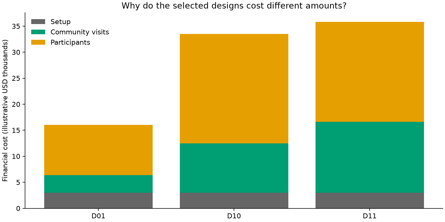
The optional cost breakdown in the appendix supports an economics discussion:

A 15-minute presentation

Minutes	Content
0–2	The decision and the two population groups
2–4	Design factors and competing objectives
4–6	One visible Study definition and a live run
6–10	Budget and Pareto plots
10–12	Priorities and an optional budget change
12–13	Assumptions a real project would replace
13–15	Discussion

The notebook's setup cells are collapsed, and slideshow metadata identifies the main narrative and its figures. The model details and cost breakdown are technical appendices. Use this guide's running order and budget/priority changes to prepare the presentation; saved notebook outputs and HTML support a version without live execution.

What a real project would replace

Replace the synthetic population with context-specific prevalence, clustering, nonresponse and sampling-frame assumptions; add validated assay characteristics and uncertainty; use local financial and economic costs; and define objectives and practical constraints with stakeholders. The example holds assay effects fixed and does not equate antibody-status prevalence with complete protection. Communities are sampled without selection bias by construction. Real selection and nonresponse can introduce bias that more simulation cannot remove.

The notebook's references link to related serosurveillance work and its costing literature. They provide context for the scientific question; the numerical assumptions are illustrative.

Export the results

From a notebook code cell, export the per-design scores and decision metadata:

report.summary.to_dataframe(include_metadata=True).to_csv(
    "serosurvey_designs.csv", index=False
)

To regenerate documentation figures:

uv run --extra notebook python examples/serosurvey_study.py