Reactor Design Study

This tutorial walks through a multi-phase trade study for a continuous stirred-tank reactor (CSTR) with competing objectives. The reactor model uses closed-form Arrhenius kinetics — no dependencies beyond numpy.

Run it yourself

The full runnable script is at examples/cstr_study.py.

uv run python examples/cstr_study.py

The problem

A continuous stirred-tank reactor (CSTR) is a standard unit operation in chemical engineering. Reactants flow in continuously, mix perfectly inside the vessel, and products flow out at steady state.

We model two series reactions:

\[A \xrightarrow{k_1} B \xrightarrow{k_2} C\]

where B is the desired product and C is an unwanted byproduct. Each rate constant follows the Arrhenius law:

\[k_i = A_i \exp\!\left(-\frac{E_{a,i}}{R\,T}\right)\]

At steady state, the CSTR mass balance gives the exit concentrations:

\[C_A = \frac{C_{A,\text{in}}}{1 + k_1 \tau}, \qquad C_B = \frac{k_1 \tau \, C_{A,\text{in}}}{(1 + k_1 \tau)(1 + k_2 \tau)}\]

where \(\tau\) is the mean residence time. From these we define:

• Conversion: \(X = 1 - C_A / C_{A,\text{in}}\) — fraction of A consumed (higher is better).
• Selectivity: \(S = C_B / (C_{A,\text{in}} - C_A)\) — fraction of converted A that became the desired product B (higher is better).
• Energy cost: \(0.01(T - 300)^2 + 5 \dot{V}_c\) — a simplified model of heating plus coolant pumping costs (lower is better).

Why the objectives conflict

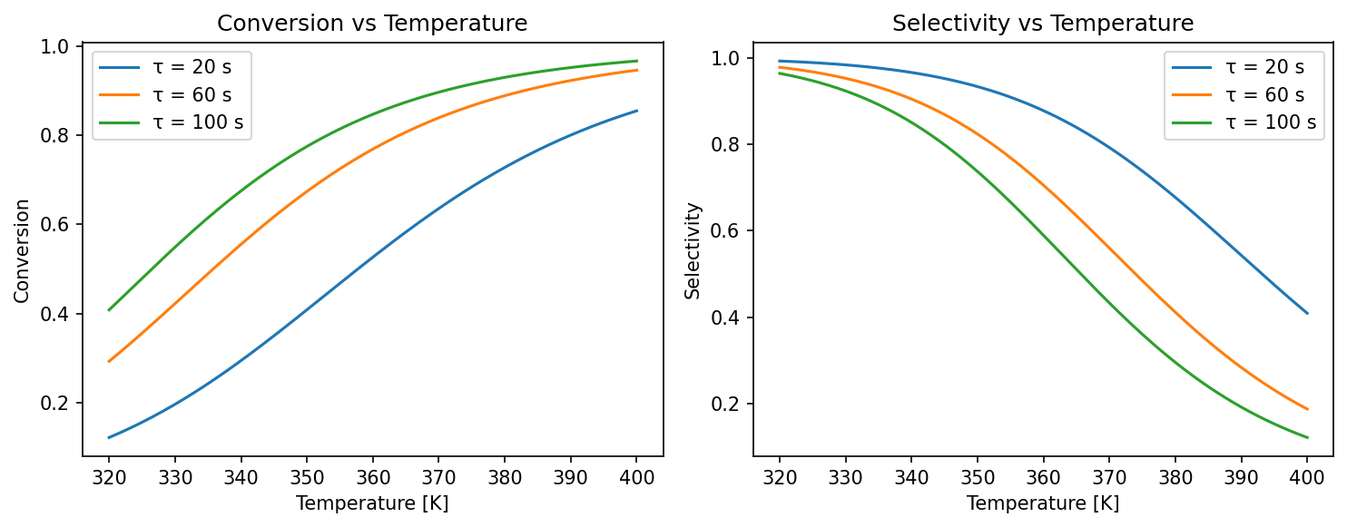
Raising the reactor temperature increases \(k_1\) (better conversion), but also accelerates the unwanted \(B \to C\) reaction because \(E_{a,2} > E_{a,1}\), which hurts selectivity. Meanwhile, both heating and cooling cost energy. There is no single set of operating conditions that simultaneously maximizes conversion and selectivity while minimizing cost — the solutions lie on a Pareto front.

The kinetics plot below shows this conflict directly. Conversion rises monotonically with temperature, but selectivity peaks and then falls as the consecutive \(B \to C\) reaction accelerates:

Ground-truth model

The code below implements the steady-state equations as a pure Python function. Because the model is closed-form, every evaluation takes microseconds — ideal for demonstrating trade-study without waiting for expensive simulations.

# A -> B -> C  (series reactions, B is the desired product)
# rate1 = k1 * C_A,  rate2 = k2 * C_B
# k_i = A_i * exp(-Ea_i / (R * T))

A1 = 1e6  # pre-exponential factor, reaction 1 [1/s]
A2 = 1e8  # pre-exponential factor, reaction 2 [1/s]
EA1 = 5e4  # activation energy, reaction 1 [J/mol]
EA2 = 7e4  # activation energy, reaction 2 [J/mol]
R_GAS = 8.314  # universal gas constant [J/(mol·K)]


def cstr_steady_state(
    temperature: float,
    residence_time: float,
    inlet_concentration: float,
    coolant_flow: float,
) -> dict[str, float]:
    """Compute steady-state CSTR outputs.

    Args:
        temperature: Reactor temperature [K].
        residence_time: Mean residence time [s].
        inlet_concentration: Inlet concentration of A [mol/L].
        coolant_flow: Coolant flow rate [L/s] (affects energy cost).

    Returns:
        Dictionary with conversion, selectivity, and energy_cost.
    """
    k1 = A1 * math.exp(-EA1 / (R_GAS * temperature))
    k2 = A2 * math.exp(-EA2 / (R_GAS * temperature))

    tau = residence_time
    ca = inlet_concentration / (1.0 + k1 * tau)
    cb = (k1 * tau * inlet_concentration) / ((1.0 + k1 * tau) * (1.0 + k2 * tau))

    conversion = 1.0 - ca / inlet_concentration
    selectivity = cb / (inlet_concentration - ca) if conversion > 1e-12 else 0.0

    # Energy cost: heating + coolant pumping (simplified)
    energy_cost = 0.01 * (temperature - 300.0) ** 2 + 5.0 * coolant_flow

    return {
        "conversion": conversion,
        "selectivity": selectivity,
        "energy_cost": energy_cost,
    }

Simulator and scorer

trade-study uses two protocols:

• A Simulator produces (truth, observations) pairs — here, the truth is the exact steady-state output and the observations add 2 % Gaussian noise to simulate real measurement uncertainty.
• A Scorer extracts the objective values that will populate the results table.

class CSTRSimulator:
    """Ground-truth CSTR simulator (Simulator protocol)."""

    def generate(self, config: dict[str, Any]) -> tuple[Any, Any]:
        """Generate ground truth and noisy observations.

        Args:
            config: Must contain temperature, residence_time,
                inlet_concentration, and coolant_flow.

        Returns:
            Tuple of (truth_dict, noisy_observations_dict).
        """
        truth = cstr_steady_state(
            temperature=config["temperature"],
            residence_time=config["residence_time"],
            inlet_concentration=config["inlet_concentration"],
            coolant_flow=config["coolant_flow"],
        )
        rng = np.random.default_rng(hash(frozenset(config.items())) % 2**32)
        noisy = {
            k: max(0.0, v + rng.normal(0, 0.02 * abs(v) + 1e-6))
            for k, v in truth.items()
        }
        return truth, noisy


class CSTRScorer:
    """Score CSTR outputs (Scorer protocol)."""

    def score(
        self,
        truth: Any,
        observations: Any,
        config: dict[str, Any],
    ) -> dict[str, float]:
        """Return observed values as scores.

        Args:
            truth: Ground truth dict (unused — we score observations).
            observations: Noisy observations dict.
            config: Trial configuration (unused).

        Returns:
            Scores for each observable.
        """
        return {
            "conversion": observations["conversion"],
            "selectivity": observations["selectivity"],
            "energy_cost": observations["energy_cost"],
        }

Define observables and factors

Observables declare what we measure and which direction is better. Each one becomes a column in the results table.

observables = [
    Observable("conversion", Direction.MAXIMIZE),
    Observable("selectivity", Direction.MAXIMIZE),
    Observable("energy_cost", Direction.MINIMIZE),
]

Factors declare what we can control — here, four continuous operating parameters with physical bounds:

factors = [
    Factor("temperature", FactorType.DISCRETE, levels=[330, 350, 370, 390]),
    Factor("residence_time", FactorType.DISCRETE, levels=[20, 50, 80, 110]),
    Factor("inlet_concentration", FactorType.DISCRETE, levels=[0.5, 1.5, 2.5]),
    Factor("coolant_flow", FactorType.DISCRETE, levels=[1.0, 3.0]),
]

Constraints

Hard feasibility bounds can be defined with Constraint objects. feasibility_filter builds a phase filter that drops designs violating any constraint:

# Require conversion >= 0.50 and energy cost <= 100
min_conversion = Constraint(
    name="min_conversion",
    observable="conversion",
    op=">=",
    threshold=0.50,
)
max_energy = Constraint(
    name="max_energy",
    observable="energy_cost",
    op="<=",
    threshold=100.0,
)

Factor screening

Before committing to a full grid sweep, Sobol screening identifies which factors influence the objectives most:

    world = CSTRSimulator()
    scorer = CSTRScorer()

    # Screening requires continuous factors; define ranges matching the
    # discrete levels so SALib can build its sample matrix.
    screening_factors = [
        Factor("temperature", FactorType.CONTINUOUS, bounds=(330.0, 390.0)),
        Factor("residence_time", FactorType.CONTINUOUS, bounds=(20.0, 110.0)),
        Factor("inlet_concentration", FactorType.CONTINUOUS, bounds=(0.5, 2.5)),
        Factor("coolant_flow", FactorType.CONTINUOUS, bounds=(1.0, 3.0)),
    ]

    def run_fn(config: dict[str, Any]) -> dict[str, float]:
        """Compose simulator + scorer for screening.

        Returns:
            Score dictionary from the scorer.
        """
        truth, obs = world.generate(config)
        return scorer.score(truth, obs, config)

    importance = screen(
        run_fn,
        screening_factors,
        method="sobol",
        n_trajectories=8,
        seed=42,
    )
    print("Sobol screening:")
    for name, vals in importance.items():
        print(f"  {name}: {vals}")

    reduced = reduce_factors(screening_factors, importance, threshold=0.01)
    print(f"\nImportant factors: {[f.name for f in reduced]}")

Build the study phases

A Study chains multiple Phases. Phase 1 explores the design space broadly with a 60-point Latin hypercube. The top_k_pareto_filter(20) callback selects the 20 best designs (by Pareto rank) and passes them to Phase 2. Phase 2 re-evaluates those 20 designs for confirmation (with fresh noise draws), acting as a validation step.

# Phase 1: coarse factorial sweep (96 designs)
discovery_grid = build_grid(factors, method="full")

# Phase 2: callable grid zooms in on the promising region
phases = [
    Phase(
        name="discovery",
        grid=discovery_grid,
        filter_fn=top_k_pareto_filter(40),
    ),
    Phase(
        name="refinement",
        grid=refine_grid,
    ),
]

Run and inspect results

Create a Study, call .run(), and then query results per phase:

    study = Study(
        world=CSTRSimulator(),
        scorer=CSTRScorer(),
        observables=observables,
        phases=phases,
    )
    study.run()

The results include the Pareto front, per-design scores, and the hypervolume indicator — a single number summarizing how well the front covers the objective space (higher is better):

    _print_results(study)
    _print_quality(study)

Pareto front scatter matrix

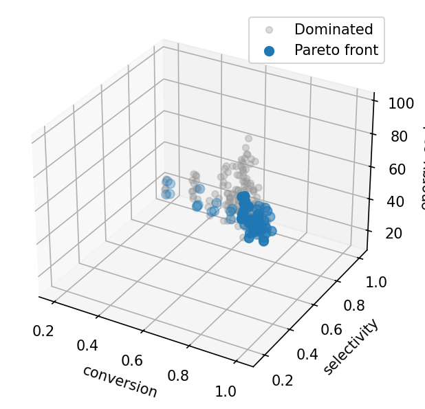
With three objectives the front is a surface; plot_front shows all pairwise projections. The conversion–selectivity panel is the classic Pareto trade-off curve.

Parallel coordinates

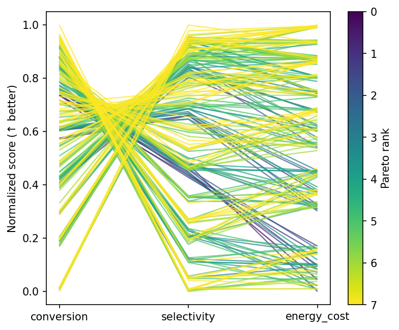
Each line is one reactor configuration, coloured by Pareto membership. Front designs cluster at moderate temperatures and longer residence times — the operating region where conversion and selectivity are both reasonable.

Selectivity strip plot

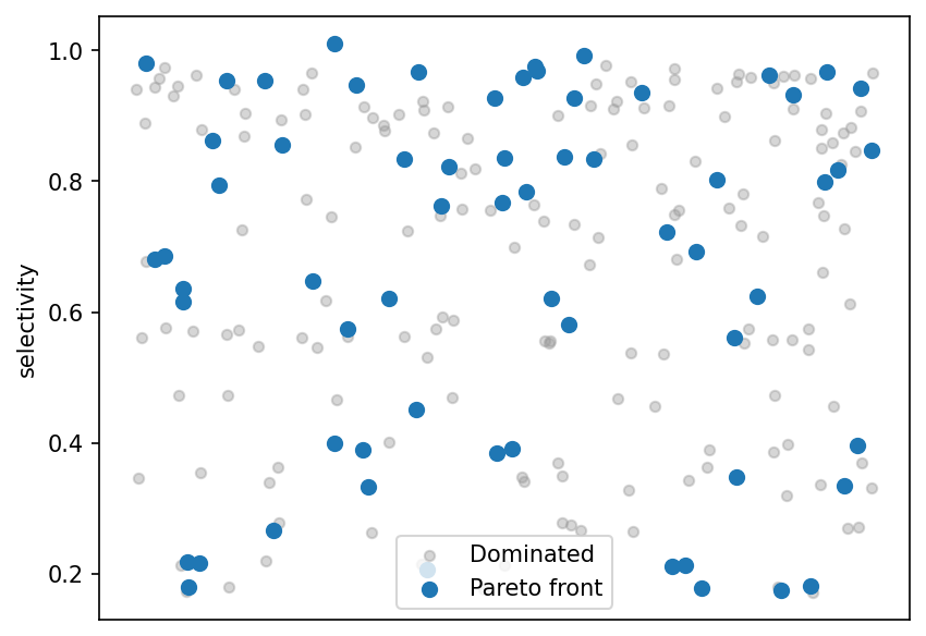
Scores for each design, split by Pareto status. Front members span the full selectivity range, reflecting different points along the conversion–selectivity trade-off.

What to try next

• Call stack_bayesian() on the Pareto front to compute model-averaging weights.
• Save results with save_results() for later analysis.
• Combine feasibility_filter with top_k_pareto_filter across successive phases for constrained multi-objective optimisation.

Progress callbacks and parallel execution

run_grid accepts a callback for progress reporting and n_jobs for parallel execution via joblib:

    from trade_study import TrialResult, run_grid

    world = CSTRSimulator()
    scorer = CSTRScorer()
    grid = build_grid(factors, method="full")

    completed = 0

    def progress(_idx: int, total: int, _result: TrialResult) -> None:
        """Print progress every 20 trials.

        Args:
            _idx: Current trial index (unused).
            total: Total number of trials.
            _result: The completed trial result (unused).
        """
        nonlocal completed
        completed += 1
        if completed % 20 == 0 or completed == total:
            print(f"  Progress: {completed}/{total} trials done")

    results = run_grid(
        world=world,
        scorer=scorer,
        grid=grid,
        observables=observables,
        n_jobs=2,
        callback=progress,
    )
    print(f"\nParallel run (n_jobs=2): {results.scores.shape[0]} trials")

Adaptive exploration

When the design space is too large for a grid sweep, use Phase(grid="adaptive") for optuna-driven multi-objective Bayesian optimisation. The factors argument on Study provides the parameter bounds:

    # Adaptive phase uses optuna NSGA-II to explore the design space
    adaptive_phases = [
        Phase(
            name="adaptive_search",
            grid="adaptive",
            n_trials=50,
            filter_fn=top_k_pareto_filter(15),
        ),
        Phase(name="validate", grid="carry"),
    ]

    study = Study(
        world=CSTRSimulator(),
        scorer=CSTRScorer(),
        observables=observables,
        phases=adaptive_phases,
        factors=factors,
    )
    study.run()

    r = study.results("validate")
    directions = [o.direction for o in observables]
    front = extract_front(r.scores, directions)
    print(f"\nAdaptive study: {r.scores.shape[0]} validated, {len(front)} on front")

Feasibility-constrained phases

Use feasibility_filter as a phase filter to enforce hard constraints before passing designs to subsequent phases:

    feas_phases = [
        Phase(
            name="sweep",
            grid=build_grid(factors, method="full"),
            filter_fn=feasibility_filter(
                constraints=[min_conversion, max_energy],
            ),
        ),
        Phase(name="feasible", grid="carry"),
    ]

    study = Study(
        world=CSTRSimulator(),
        scorer=CSTRScorer(),
        observables=observables,
        phases=feas_phases,
    )
    study.run()

    sweep_r = study.results("sweep")
    feas_r = study.results("feasible")
    print("\nFeasibility filter:")
    print(f"  {sweep_r.scores.shape[0]} total -> {feas_r.scores.shape[0]} feasible")