Bayesian Model Criticism

This tutorial walks through a scoring-and-stacking workflow for Bayesian models. It demonstrates the features that set trade-study apart from conventional hyperparameter optimizers: proper scoring rules, calibration assessment, and score-based model averaging.

The underlying model is a conjugate Bayesian linear regression — no MCMC sampler or external probabilistic programming library needed, only numpy.

Run it yourself

The full runnable script is at examples/bayesian_study.py.

uv run --extra examples python examples/bayesian_study.py

The problem

We want to fit a Bayesian regression \(y = a + bx + \varepsilon\) where \(\varepsilon \sim \mathcal{N}(0,\sigma_\text{true}^2)\) and the true coefficients are known (\(a=2\), \(b=3\), \(\sigma_\text{true}=0.5\)).

The design question is: which prior hyperparameters and sample sizes produce well-calibrated, accurate posteriors? Specifically, each configuration controls three knobs:

Factor	Meaning
prior_var	Variance of the Normal prior on \((a, b)\)
noise_scale	Assumed observation noise \(\sigma\) (may disagree with truth)
n_obs	Number of training observations

Choosing noise_scale too small produces overconfident posteriors; too large gives conservative intervals. A tight prior (prior_var small) biases the coefficients toward zero. More data always helps, but at a computational cost.

Ground-truth model

# True data-generating process:  y = a + b*x + eps,  eps ~ N(0, sigma_true^2)
TRUE_A = 2.0  # intercept
TRUE_B = 3.0  # slope
SIGMA_TRUE = 0.5  # observation noise std

N_TEST = 50  # test locations for scoring
RNG_SEED = 42

rng = np.random.default_rng(RNG_SEED)
X_TEST = np.linspace(0.0, 1.0, N_TEST)
Y_TEST = TRUE_A + TRUE_B * X_TEST + rng.normal(0.0, SIGMA_TRUE, N_TEST)

Conjugate posterior

Because we use a Normal prior with known noise variance, the posterior over regression coefficients is available in closed form. Given design matrix \(\mathbf{X}\) and prior precision \(\boldsymbol{\Lambda}_0 = \sigma_\text{prior}^{-2}\mathbf{I}\):

\[ \boldsymbol{\Sigma}_n = \left(\boldsymbol{\Lambda}_0 + \frac{\mathbf{X}^\top\mathbf{X}}{\sigma^2}\right)^{-1} \qquad \boldsymbol{\mu}_n = \boldsymbol{\Sigma}_n \frac{\mathbf{X}^\top\mathbf{y}}{\sigma^2} \]

We draw posterior predictive samples by projecting coefficient draws through the test design matrix and adding observation noise.

def bayesian_regression(
    x_train: np.ndarray,
    y_train: np.ndarray,
    prior_var: float,
    noise_scale: float,
    n_samples: int = 500,
    seed: int = RNG_SEED,
) -> tuple[np.ndarray, np.ndarray]:
    """Fit a conjugate Bayesian linear regression and draw predictions.

    Prior:  beta = (a, b) ~ N(0, prior_var * I)
    Likelihood:  y | x, beta ~ N(X @ beta, noise_scale^2 * I)

    Args:
        x_train: Training inputs, shape (n,).
        y_train: Training targets, shape (n,).
        prior_var: Prior variance for each coefficient.
        noise_scale: Assumed observation noise standard deviation.
        n_samples: Number of posterior predictive draws.
        seed: Random seed.

    Returns:
        Tuple of (posterior_mean_at_test, predictive_samples_at_test).
        posterior_mean_at_test has shape (N_TEST,).
        predictive_samples_at_test has shape (N_TEST, n_samples).
    """
    gen = np.random.default_rng(seed)

    # Design matrices
    x_design = np.column_stack([np.ones_like(x_train), x_train])  # (n, 2)
    x_star = np.column_stack([np.ones(N_TEST), X_TEST])  # (N_TEST, 2)

    sigma2 = noise_scale**2
    prior_precision = np.eye(2) / prior_var  # (2, 2)

    # Conjugate posterior:  beta | y ~ N(mu_n, Sigma_n)
    gram = x_design.T @ x_design  # X^T X
    posterior_cov = np.linalg.inv(prior_precision + gram / sigma2)
    posterior_mean = posterior_cov @ (x_design.T @ y_train / sigma2)

    # Posterior predictive at test locations
    pred_mean = x_star @ posterior_mean  # (N_TEST,)

    # Draw beta samples, then project to predictions and add noise
    beta_samples = gen.multivariate_normal(
        posterior_mean,
        posterior_cov,
        size=n_samples,
    )  # (n_samples, 2)
    pred_samples = (x_star @ beta_samples.T) + gen.normal(
        0.0, noise_scale, (N_TEST, n_samples)
    )

    return pred_mean, pred_samples

Simulator and scorer

The simulator generates training data from the true model, fits the conjugate posterior, and returns posterior predictive samples at held-out test locations. The scorer evaluates three complementary metrics:

• CRPS (Continuous Ranked Probability Score) — a proper scoring rule that rewards sharp, well-calibrated predictive distributions.
• Energy score — a multivariate proper scoring rule complementary to CRPS.
• Coverage (95 %) — the fraction of test points whose true value falls inside the 95 % posterior predictive interval.
• RMSE — root mean squared error of the posterior mean.
• MAE — mean absolute error of the posterior mean.

class BayesianRegressionSimulator:
    """Generate training data and compute the Bayesian posterior.

    Each config specifies prior hyperparameters and sample size.
    The "truth" is the held-out test set; "observations" are the
    posterior predictive samples at those test points.

    Args:
        n_samples: Number of posterior predictive draws.  Fewer draws
            give faster but noisier score estimates — useful as a cheap
            surrogate in a multi-fidelity workflow.
    """

    def __init__(self, n_samples: int = 500) -> None:
        """Initialise the simulator.

        Args:
            n_samples: Number of posterior predictive draws.
        """
        self.n_samples = n_samples

    def generate(self, config: dict[str, Any]) -> tuple[Any, Any]:
        """Draw training data, fit posterior, and return test predictions.

        Args:
            config: Must contain prior_var, noise_scale, n_obs.

        Returns:
            Tuple of (y_test, observation dict with predictive samples
            and posterior mean predictions).
        """
        gen = np.random.default_rng(RNG_SEED)
        n_obs = round(config["n_obs"])

        # Draw training data from the true model
        x_train = gen.uniform(0.0, 1.0, n_obs)
        y_train = TRUE_A + TRUE_B * x_train + gen.normal(0.0, SIGMA_TRUE, n_obs)

        # Compute conjugate posterior
        pred_mean, pred_samples = bayesian_regression(
            x_train,
            y_train,
            prior_var=config["prior_var"],
            noise_scale=config["noise_scale"],
            n_samples=self.n_samples,
        )

        observations = {
            "pred_mean": pred_mean,
            "pred_samples": pred_samples,
            "n_obs": n_obs,
        }
        return Y_TEST, observations


class BayesianRegressionScorer:
    """Score posterior predictions with proper scoring rules."""

    def score(
        self,
        truth: Any,
        observations: Any,
        config: dict[str, Any],
    ) -> dict[str, float]:
        """Compute CRPS, energy, 95 percent coverage, RMSE, and MAE.

        Args:
            truth: True test-set values (y_test).
            observations: Dict with pred_samples and pred_mean arrays.
            config: Hyperparameter dict (unused).

        Returns:
            Scores for crps, energy, coverage_95, rmse, and mae.
        """
        crps_val = score("crps", observations["pred_samples"], truth)
        energy_val = score("energy", observations["pred_samples"], truth)
        cov95 = score("coverage", observations["pred_samples"], truth, level=0.95)
        rmse_val = score("rmse", observations["pred_mean"], truth)
        mae_val = score("mae", observations["pred_mean"], truth)
        return {
            "crps": crps_val,
            "energy": energy_val,
            "coverage_95": cov95,
            "rmse": rmse_val,
            "mae": mae_val,
        }

Observables and factors

Coverage is given lower weight (0.5) because a model can trivially achieve 100 % coverage by being very wide; CRPS already penalises that.

observables = [
    Observable("crps", Direction.MINIMIZE),
    Observable("energy", Direction.MINIMIZE, weight=0.5),
    Observable("coverage_95", Direction.MAXIMIZE, weight=0.5),
    Observable("rmse", Direction.MINIMIZE),
    Observable("mae", Direction.MINIMIZE, weight=0.3),
]

factors = [
    Factor("prior_var", FactorType.CONTINUOUS, bounds=(0.1, 10.0)),
    Factor("noise_scale", FactorType.CONTINUOUS, bounds=(0.1, 2.0)),
    Factor("n_obs", FactorType.CONTINUOUS, bounds=(10.0, 200.0)),
]

Annotations

An Annotation attaches external metadata — here, a simple linear cost model for the number of observations:

compute_cost = Annotation(
    name="compute_cost",
    lookup=lambda n: float(n) * 0.01,
    key="n_obs",
)

Constraints

A Constraint defines a hard feasibility bound on an observable. feasibility_filter builds a phase filter that drops any design violating the constraints:

# Require at least 90% empirical coverage at the 95% nominal level
min_coverage = Constraint(
    name="min_coverage",
    observable="coverage_95",
    op=">=",
    threshold=0.90,
)

Factor screening

Before running the full grid, Morris screening identifies which factors influence the scores most. reduce_factors drops any factor whose \(\mu^*\) falls below a threshold:

    def run_fn(config: dict[str, Any]) -> dict[str, float]:
        """Compose simulator + scorer for screening.

        Returns:
            Score dictionary from the scorer.
        """
        config = {**config, "n_obs": round(config["n_obs"])}
        truth, obs = world.generate(config)
        return scorer.score(truth, obs, config)

    importance = screen(run_fn, factors, method="morris", n_trajectories=8, seed=42)
    print("Morris screening (mu_star):")
    for name, vals in importance.items():
        print(f"  {name}: {vals}")

    reduced = reduce_factors(factors, importance, threshold=0.01)
    print(f"\nImportant factors (threshold=0.01): {[f.name for f in reduced]}")

Grid evaluation

A 60-point Latin hypercube covers the three-factor space. run_grid evaluates every configuration and collects scores and annotations into a ResultsTable:

    grid = build_grid(factors, method="lhs", n_samples=60, seed=42)
    for cfg in grid:
        cfg["n_obs"] = round(cfg["n_obs"])

    print(f"\nLHS grid: {len(grid)} configurations")

    results = run_grid(
        world=world,
        scorer=scorer,
        grid=grid,
        observables=observables,
        annotations=[compute_cost],
    )

Pareto analysis

    print(f"\nPareto front: {len(front_idx)} / {results.scores.shape[0]} designs")

    header = (
        f"{'prior_var':>10s}  {'noise':>6s}  {'n_obs':>5s}  "
        f"{'CRPS':>6s}  {'Energy':>7s}  {'Cov95':>6s}  "
        f"{'RMSE':>6s}  {'MAE':>6s}  {'Cost':>5s}"
    )
    print(f"\n{header}")
    print("-" * len(header))
    for i in front_idx:
        cfg = results.configs[i]
        crps_val = results.scores[i, 0]
        energy_val = results.scores[i, 1]
        cov = results.scores[i, 2]
        rmse_val = results.scores[i, 3]
        mae_val = results.scores[i, 4]
        cost = results.annotations[i, 0] if results.annotations is not None else 0.0
        print(
            f"{cfg['prior_var']:10.2f}  {cfg['noise_scale']:6.2f}  "
            f"{cfg['n_obs']:5d}  "
            f"{crps_val:6.3f}  {energy_val:7.3f}  {cov:6.3f}  "
            f"{rmse_val:6.3f}  {mae_val:6.3f}  {cost:5.1f}"
        )

Pareto front scatter matrix

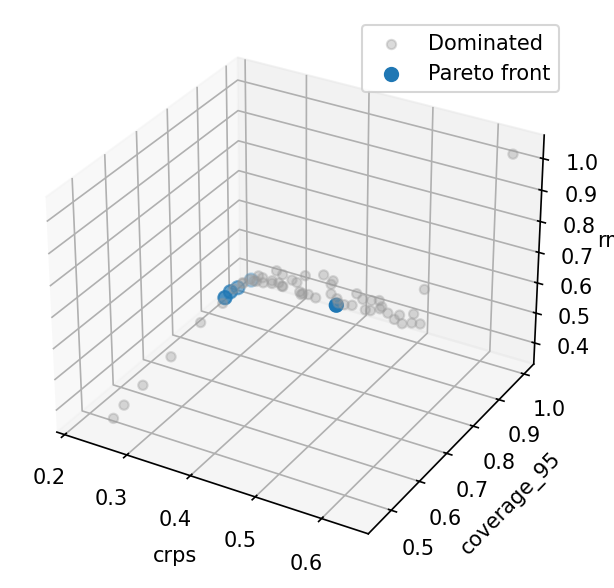
With three objectives the front is a surface; plot_front shows all pairwise projections. Models with low CRPS generally have good coverage and low RMSE, but there are trade-offs when noise is mis-specified.

Parallel coordinates

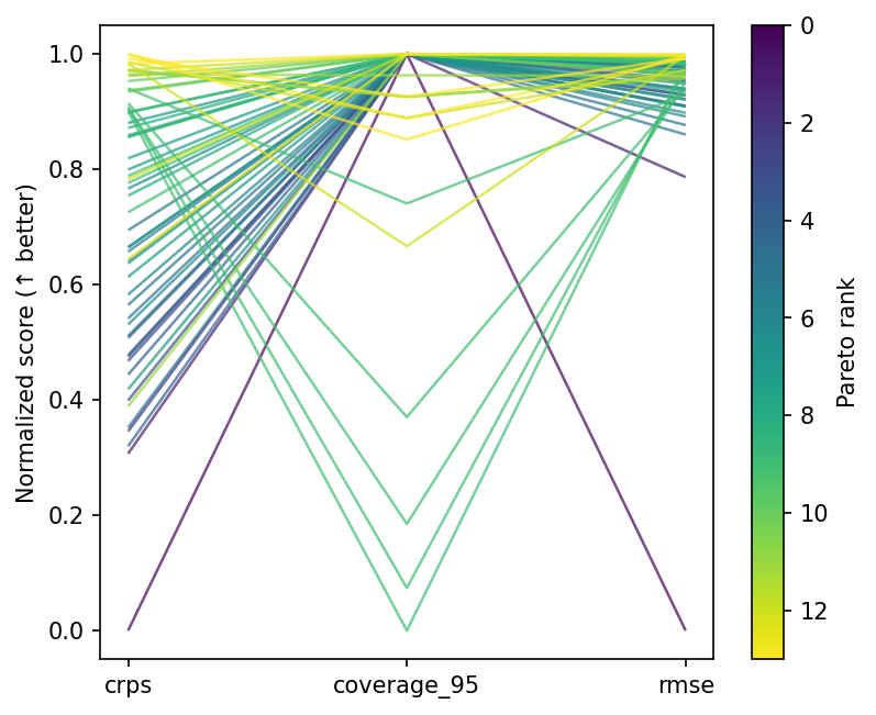
Front designs cluster at moderate prior variance and noise scales close to the true value — the region where the model is neither overconfident nor excessively vague.

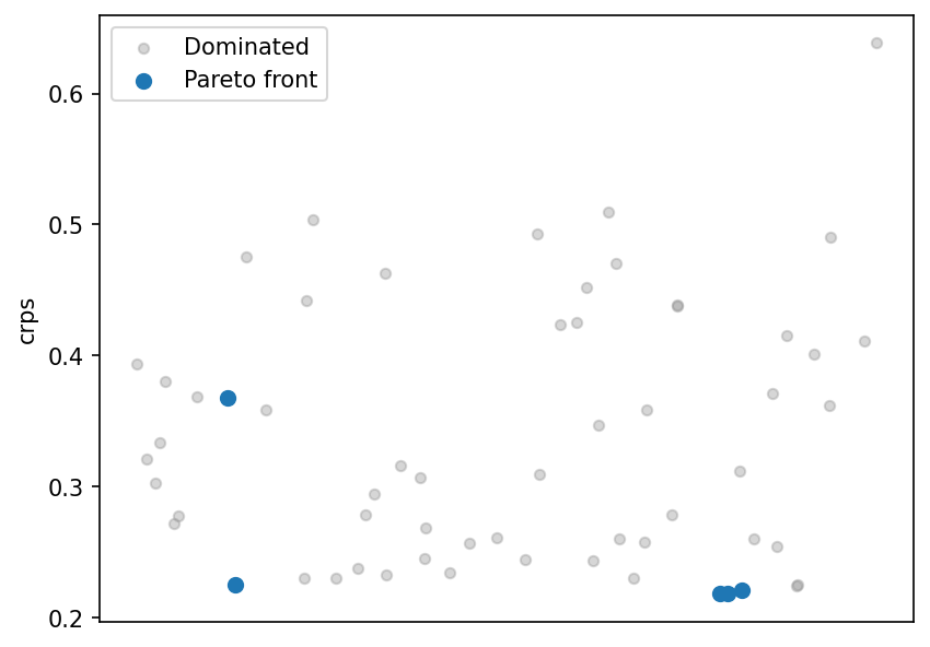
CRPS strip plot

Quality indicators

hypervolume measures the dominated volume of the Pareto front; igd_plus (inverted generational distance plus) measures how close the front is to a reference set. Together they quantify front quality — useful for comparing design methods or grid sizes:

    directions = [o.direction for o in observables]
    weights = [o.weight for o in observables]

    front_scores = results.scores[front_idx]

    # Build a synthetic reference front from per-objective best values
    n_obj = front_scores.shape[1]
    ideal = np.tile(np.median(front_scores, axis=0), (n_obj, 1))
    for j, d in enumerate(directions):
        ideal[j, j] = (
            front_scores[:, j].min()
            if d == Direction.MINIMIZE
            else front_scores[:, j].max()
        )

    ref_point = np.array([
        front_scores[:, j].max()
        if d == Direction.MINIMIZE
        else front_scores[:, j].min()
        for j, d in enumerate(directions)
    ])
    hv = hypervolume(front_scores, ref_point, directions, weights)
    igd = igd_plus(front_scores, ideal, directions, weights)
    print(f"\nHypervolume: {hv:.4f}")
    print(f"IGD+:        {igd:.4f}")

Feasibility filtering

Apply Constraint + feasibility_filter to keep only designs meeting hard bounds (here, coverage_95 >= 0.90):

    all_idx = np.arange(results.scores.shape[0])
    feas_filter = feasibility_filter(constraints=[min_coverage])
    kept = feas_filter(results, observables)
    print("\nFeasibility filter (coverage_95 >= 0.90):")
    print(f"  {len(all_idx)} total -> {len(kept)} feasible designs")

Weighted-sum filtering

weighted_sum_filter scalarises objectives into a single score via min-max normalisation and weighted combination, then keeps the top-K designs. Useful when you want a simple ranking without full Pareto analysis:

    ws_filter = weighted_sum_filter(
        weights={"crps": 1.0, "coverage_95": 0.5, "rmse": 0.8},
        k=8,
    )
    kept = ws_filter(results, observables)
    print("\nWeighted-sum filter (top 8 by scalarised score):")
    for i in kept[:5]:
        cfg = results.configs[i]
        print(
            f"  prior_var={cfg['prior_var']:.2f}, "
            f"noise={cfg['noise_scale']:.2f}, "
            f"n_obs={cfg['n_obs']}"
        )
    if len(kept) > 5:
        print(f"  ... and {len(kept) - 5} more")

Sobol grid

build_grid(method="sobol") generates quasi-random points with better space-filling properties than LHS for low dimensions:

    sobol_grid = build_grid(factors, method="sobol", n_samples=40, seed=0)
    for cfg in sobol_grid:
        cfg["n_obs"] = round(cfg["n_obs"])

    print(f"\nSobol grid: {len(sobol_grid)} configurations")
    sobol_results = run_grid(
        world=world,
        scorer=scorer,
        grid=sobol_grid,
        observables=observables,
    )
    directions = [o.direction for o in observables]
    weights = [o.weight for o in observables]
    sobol_front = extract_front(sobol_results.scores, directions, weights)
    print(f"Sobol Pareto front: {len(sobol_front)} designs")

Study workflow

The Study class orchestrates multi-phase workflows. Study.summary() returns per-phase statistics and Study.stack() computes stacking weights directly:

    world = BayesianRegressionSimulator()
    scorer = BayesianRegressionScorer()

    grid = build_grid(factors, method="lhs", n_samples=60, seed=42)
    for cfg in grid:
        cfg["n_obs"] = round(cfg["n_obs"])

    study = Study(
        world=world,
        scorer=scorer,
        observables=observables,
        phases=[
            Phase(
                name="explore",
                grid=grid,
                filter_fn=feasibility_filter(
                    constraints=[min_coverage],
                ),
            ),
            Phase(name="rank", grid="carry"),
        ],
        annotations=[compute_cost],
    )
    study.run()

    # Study.summary() — per-phase statistics
    summary = study.summary()
    for phase_name, stats in summary.items():
        print(f"\n  Phase '{phase_name}':")
        print(f"    trials={stats['n_trials']}, front={stats['n_front']}")
        for obs_name, rng in stats["observable_ranges"].items():
            print(f"    {obs_name}: [{rng['min']:.4f}, {rng['max']:.4f}]")

    # Study.stack() — convenience method for score-based stacking
    stacking_w = study.stack("rank", maximize=False)
    print("Study.stack() weights (top entries):")
    for i, w in enumerate(stacking_w):
        if w > 0.01:
            print(f"  design {i}: {w:.3f}")

Score-based stacking

stack_scores finds simplex-constrained weights that minimise the composite MSE across test points. The stacked ensemble often beats every individual model because it smooths over prior mis-specification:

    # Build a score matrix from the front: per-test-point squared errors
    front_predictions = []
    score_matrix_rows = []
    for i in front_idx:
        cfg = results.configs[i]
        _, obs = world.generate(cfg)
        front_predictions.append(obs["pred_mean"])
        sq_errors = (obs["pred_mean"] - Y_TEST) ** 2
        score_matrix_rows.append(sq_errors)

    score_mat = np.array(score_matrix_rows)  # (n_front, n_test)
    stacking_weights = stack_scores(score_mat, maximize=False)
    print("\nStacking weights (MSE-optimal):")
    for idx, w in zip(front_idx, stacking_weights, strict=True):
        if w > 0.01:
            cfg = results.configs[idx]
            print(
                f"  prior_var={cfg['prior_var']:.2f}, "
                f"noise={cfg['noise_scale']:.2f}, "
                f"n_obs={cfg['n_obs']}: w={w:.3f}"
            )

    ens_mean = ensemble_predict(front_predictions, stacking_weights)
    ens_rmse = float(np.sqrt(np.mean((ens_mean - Y_TEST) ** 2)))
    best_single = float(results.scores[front_idx, 3].min())  # rmse column
    print(f"\nBest single-model RMSE: {best_single:.4f}")
    print(f"Stacked ensemble RMSE:  {ens_rmse:.4f}")

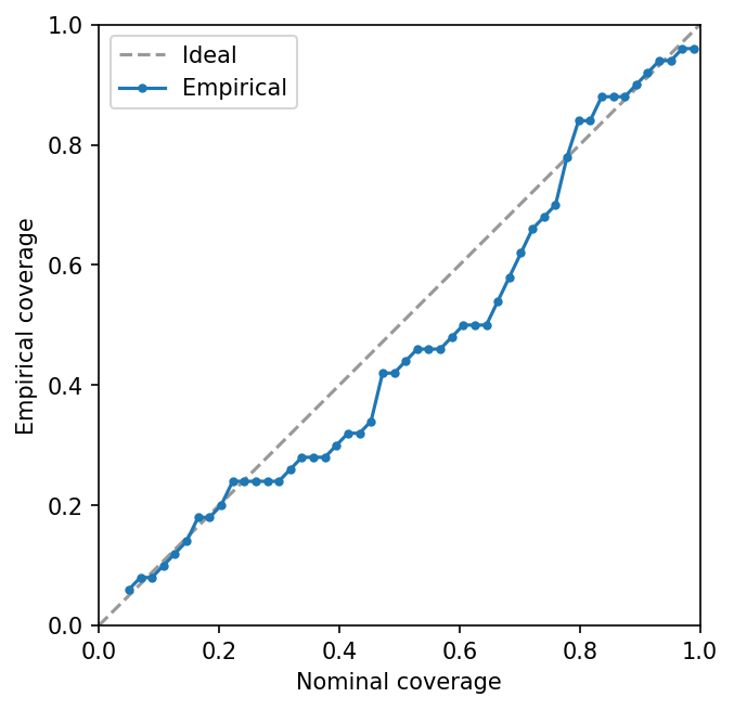
Calibration assessment

coverage_curve evaluates empirical coverage at many nominal levels. A well-calibrated model tracks the diagonal:

    best_crps_idx = front_idx[int(np.argmin(results.scores[front_idx, 0]))]
    best_cfg = results.configs[best_crps_idx]
    _, best_obs = world.generate(best_cfg)
    nominal, empirical = coverage_curve(best_obs["pred_samples"], Y_TEST)
    pv = best_cfg["prior_var"]
    print(f"\nCalibration (best CRPS, prior_var={pv:.2f}):")
    for level in (0.5, 0.9, 0.95):
        closest = empirical[np.argmin(np.abs(nominal - level))]
        print(f"  Nominal {level:.0%}  -> Empirical {closest:.1%}")

Persistence

save_results writes the ResultsTable to disk; load_results reconstructs it. Useful for expensive studies where you want to separate evaluation from analysis:

    with tempfile.TemporaryDirectory() as tmp:
        save_results(results, tmp)
        loaded = load_results(tmp)
        n_saved = loaded.scores.shape[0]
        print(f"\nSaved and reloaded {n_saved} results successfully.")

Multi-fidelity workflow

Real-world studies often have an expensive simulator — full MCMC, a fine-mesh CFD solver, or an agent-based epidemiological model. Running every candidate design at full fidelity is wasteful. A multi-fidelity strategy screens many designs cheaply, then validates only the promising ones at high fidelity.

Phase supports this via optional world and scorer overrides. When set, a phase uses its own simulator instead of the Study-level default. Here the cheap surrogate draws only 50 posterior samples (fast but noisy CRPS estimates), while the validation phase draws 2 000:

    # Cheap surrogate: only 50 posterior draws (fast, noisier scores)
    cheap_world = BayesianRegressionSimulator(n_samples=50)
    # Expensive model: 2000 posterior draws (slow, precise scores)
    expensive_world = BayesianRegressionSimulator(n_samples=2000)

    # Phase-level scorer override: use a separate scorer for screening
    screen_scorer = BayesianRegressionScorer()
    validate_scorer = BayesianRegressionScorer()

    grid = build_grid(factors, method="lhs", n_samples=60, seed=42)
    for cfg in grid:
        cfg["n_obs"] = round(cfg["n_obs"])

    study = Study(
        world=expensive_world,
        scorer=validate_scorer,
        observables=observables,
        phases=[
            # Phase 1: screen with cheap world AND its own scorer
            Phase(
                name="screen",
                grid=grid,
                world=cheap_world,
                scorer=screen_scorer,
                filter_fn=top_k_pareto_filter(k=10),
            ),
            # Phase 2: validate top 10 with the expensive model + default scorer
            Phase(name="validate", grid="carry"),
        ],
        annotations=[compute_cost],
    )
    study.run()

    screen_r = study.results("screen")
    validate_r = study.results("validate")
    print("\nMulti-fidelity study:")
    print(f"  Screen phase:   {screen_r.scores.shape[0]} designs (50 draws)")
    print(f"  Validate phase: {validate_r.scores.shape[0]} designs (2000 draws)")

    directions = [o.direction for o in observables]
    weights = [o.weight for o in observables]
    front_idx = extract_front(validate_r.scores, directions, weights)
    print(f"  Final Pareto front: {len(front_idx)} designs")

The Study orchestrates both phases: the first screens 60 designs with the cheap surrogate and keeps the top 10 by Pareto rank, then the second re-evaluates those 10 designs with the expensive model.

This pattern applies whenever fidelity is a computational strategy rather than a design factor:

• Epidemiology — screen surveillance designs with a deterministic ODE model, validate the best with a stochastic agent-based model.
• Engineering — coarse mesh for broad exploration, fine mesh for the Pareto front.
• Forecast model grading — fast approximate inference for screening, full HMC for final assessment.

What to try next

• Try stack_bayesian() on models that expose log-likelihood (requires arviz).
• Add more phases to the Study — e.g. a third phase that re-evaluates with even higher fidelity.
• Experiment with different weighted_sum_filter weight vectors to explore different trade-off preferences.