Monitoring Station Design

This tutorial runs a multi-objective trade study over instrument settings for a remote monitoring station. The goal is to recover a known environmental signal as faithfully as possible while keeping station cost low.

Unlike the CSTR and sklearn examples — where the experiment changes what is built or trained — here the experiment changes how you observe. The underlying signal is fixed; only the instrument configuration varies.

Run it yourself

The full runnable script is at examples/monitoring_study.py.

uv run python examples/monitoring_study.py

The problem

A reference environmental signal is measured at a remote station. The instrument settings — sample rate, ADC resolution, sensor quality, and number of co-located sensors — determine how faithfully the true signal is recovered and how much the station costs.

Reference signal

A synthetic 24-hour signal with three components (numpy only):

• Diurnal cycle: smooth sinusoid with a 24-hour period.
• Short-period oscillations: two higher-frequency modes at periods of 5 minutes and 20 minutes (e.g. tidal harmonics, turbulence).
• Correlated noise: an AR(1) process (\(\varphi = 0.995\), decorrelation time \(\approx 200\) s) representing natural variability.

The signal is generated at 1-second resolution — \(N = 86\,400\) samples for a full day.

Observation model

The instrument applies a chain of realistic transformations:

1. Anti-alias filter — brick-wall low-pass at the Nyquist frequency of the configured sample rate.
2. Decimation — subsample to the configured interval.
3. Quantization — finite ADC resolution maps continuous values to \(2^b\) discrete levels.
4. Sensor noise — additive Gaussian noise whose standard deviation depends on sensor grade, reduced by \(\sqrt{n}\) averaging when multiple co-located sensors are used.

Why the objectives conflict

• Faster sampling + more bits + better sensors + more averaging → near-perfect recovery, but station cost explodes.
• Cheap configurations (300 s interval, 8-bit, field-grade, 1 sensor) lose the short-period oscillations entirely and quantize the diurnal cycle into visible steps.
• Mid-range configs face a genuine Pareto trade-off: you can spend your budget on temporal resolution or sensor quality, but rarely both.

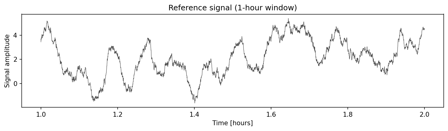
Reference signal generation

The plot below shows a 1-hour window of the latent truth, revealing the diurnal trend, the short-period oscillations, and the correlated noise component:

DURATION = 86400.0  # 24 hours [s]
DT_TRUE = 1.0  # true signal resolution [s]
N_TRUE = int(DURATION / DT_TRUE)
T_TRUE = np.arange(N_TRUE) * DT_TRUE  # time axis [s]

RNG = np.random.default_rng(42)


def generate_reference_signal() -> np.ndarray:
    """Build a synthetic 24-hour environmental signal.

    Components:
      - Diurnal cycle (period = 24 h)
      - Short-period oscillations (periods ≈ 5 min, 20 min)
      - Correlated noise (AR(1), φ = 0.995)

    Returns:
        1-D array of length N_TRUE.
    """
    t_hours = T_TRUE / 3600.0

    # Diurnal
    diurnal = 5.0 * np.sin(2.0 * np.pi * t_hours / 24.0)

    # Short-period oscillations (5 min and 20 min)
    t_min = T_TRUE / 60.0
    short = 1.2 * np.sin(2.0 * np.pi * t_min / 5.0) + 0.8 * np.cos(
        2.0 * np.pi * t_min / 20.0
    )

    # Correlated noise  (AR(1), φ = 0.995 → decorrelation ~ 200 s)
    phi = 0.995
    noise = np.empty(N_TRUE)
    noise[0] = RNG.normal()
    for i in range(1, N_TRUE):
        noise[i] = phi * noise[i - 1] + RNG.normal(scale=np.sqrt(1 - phi**2))

    return diurnal + short + noise


REFERENCE = generate_reference_signal()

Observation model

The observe() function implements the four-stage signal chain described above. Each stage is a few lines of numpy:

SENSOR_NOISE: dict[str, float] = {
    "field": 1.0,
    "lab": 0.1,
    "reference": 0.01,
}


def observe(
    signal: np.ndarray,
    sample_interval: int,
    adc_bits: int,
    sensor_grade: str,
    n_sensors: int,
    rng: np.random.Generator,
) -> np.ndarray:
    """Apply the instrument signal chain to a reference signal.

    Steps:
      1. Anti-alias low-pass filter (brick-wall in frequency domain).
      2. Decimation to the configured sample interval.
      3. Quantization to *adc_bits* resolution.
      4. Additive sensor noise, reduced by √n_sensors averaging.

    Args:
        signal: High-resolution reference signal.
        sample_interval: Seconds between samples (decimation factor).
        adc_bits: ADC bit depth.
        sensor_grade: One of "field", "lab", "reference".
        n_sensors: Number of co-located sensors to average.
        rng: Numpy random generator for reproducibility.

    Returns:
        Degraded observation array at the decimated sample rate.
    """
    # 1. Anti-alias filter (brick-wall at Nyquist of decimated rate)
    spectrum = np.fft.rfft(signal)
    freqs = np.fft.rfftfreq(len(signal), d=DT_TRUE)
    nyquist = 0.5 / sample_interval
    spectrum[freqs > nyquist] = 0.0
    filtered = np.fft.irfft(spectrum, n=len(signal))

    # 2. Decimate
    decimated = filtered[::sample_interval]

    # 3. Quantize
    sig_range = float(np.ptp(signal)) * 1.1  # 10 % headroom
    n_levels = 2**adc_bits
    step = sig_range / n_levels
    mid = float(np.mean(signal))
    quantized = np.round((decimated - mid) / step) * step + mid

    # 4. Sensor noise (averaged over n_sensors)
    sigma = SENSOR_NOISE[sensor_grade] / np.sqrt(n_sensors)
    return quantized + rng.normal(scale=sigma, size=len(quantized))

Simulator and scorer

The Simulator applies the observation model with a per-config deterministic seed. The Scorer computes three objectives:

Observable	Direction	What it measures
RMSE	minimize	RMS error after interpolating back to the reference grid
Spectral fidelity	maximize	Fraction of spectral power recovered in the 10 min – 2 h band
Station cost	minimize	Additive cost model over sample rate, ADC, grade, and sensor count

class StationSimulator:
    """Simulator that applies the instrument signal chain.

    Returns the full-resolution reference signal as 'truth' and
    the degraded, decimated observations as 'observations'.
    """

    def generate(self, config: dict[str, Any]) -> tuple[Any, Any]:
        """Generate truth and degraded observations.

        Args:
            config: Must contain sample_interval, adc_bits,
                sensor_grade, and n_sensors.

        Returns:
            Tuple of (reference_signal, degraded_observations).
        """
        seed = hash(frozenset(config.items())) % 2**32
        rng = np.random.default_rng(seed)
        obs = observe(
            REFERENCE,
            sample_interval=config["sample_interval"],
            adc_bits=config["adc_bits"],
            sensor_grade=config["sensor_grade"],
            n_sensors=config["n_sensors"],
            rng=rng,
        )
        return REFERENCE, {"observations": obs, "interval": config["sample_interval"]}


def _spectral_fidelity(truth: np.ndarray, reconstructed: np.ndarray) -> float:
    """Fraction of spectral power recovered in the 2.5-30 min band.

    Args:
        truth: Full-resolution reference signal.
        reconstructed: Signal interpolated back to the reference grid.

    Returns:
        Power ratio clamped to [0, 1].
    """
    ref_psd = np.abs(np.fft.rfft(truth)) ** 2
    rec_psd = np.abs(np.fft.rfft(reconstructed)) ** 2
    freqs = np.fft.rfftfreq(len(truth), d=DT_TRUE)
    band = (freqs >= 1 / 1800) & (freqs <= 1 / 150)  # 2.5 min - 30 min
    ref_power = float(np.sum(ref_psd[band]))
    rec_power = float(np.sum(rec_psd[band]))
    return min(rec_power / ref_power, 1.0) if ref_power > 0 else 0.0


def _station_cost(config: dict[str, Any]) -> float:
    """Additive cost model over instrument settings.

    Args:
        config: Instrument configuration dict.

    Returns:
        Total station cost in arbitrary units.
    """
    rate_cost = {1: 50, 5: 30, 15: 15, 60: 5, 300: 1}
    bits_cost = {8: 1, 12: 5, 16: 20, 24: 80}
    grade_cost = {"field": 10, "lab": 50, "reference": 200}
    return float(
        rate_cost[config["sample_interval"]]
        + bits_cost[config["adc_bits"]]
        + grade_cost[config["sensor_grade"]] * config["n_sensors"]
    )


class StationScorer:
    """Score observation quality and station cost."""

    def score(
        self,
        truth: Any,
        observations: Any,
        config: dict[str, Any],
    ) -> dict[str, float]:
        """Compute RMSE, spectral fidelity, and station cost.

        Args:
            truth: Full-resolution reference signal.
            observations: Dict with degraded signal and sample interval.
            config: Instrument configuration.

        Returns:
            Scores for rmse, spectral_fidelity, and station_cost.
        """
        obs = observations["observations"]
        interval = observations["interval"]

        # Interpolate observations back to the reference grid
        obs_times = np.arange(len(obs)) * interval
        reconstructed = np.interp(T_TRUE, obs_times, obs)

        # RMSE
        rmse = float(np.sqrt(np.mean((truth - reconstructed) ** 2)))

        # Spectral fidelity: power ratio in the short-period band
        fidelity = _spectral_fidelity(truth, reconstructed)

        # Station cost (arbitrary units)
        cost = _station_cost(config)

        return {
            "rmse": rmse,
            "spectral_fidelity": fidelity,
            "station_cost": float(cost),
        }

Define observables and factors

Observables declare what we measure and which direction is better:

observables = [
    Observable("rmse", Direction.MINIMIZE),
    Observable("spectral_fidelity", Direction.MAXIMIZE),
    Observable("station_cost", Direction.MINIMIZE),
]

Factors define the instrument search space. The full factorial grid is \(5 \times 4 \times 3 \times 4 = 240\) configurations:

factors = [
    Factor("sample_interval", FactorType.DISCRETE, levels=[1, 5, 15, 60, 300]),
    Factor("adc_bits", FactorType.DISCRETE, levels=[8, 12, 16, 24]),
    Factor("sensor_grade", FactorType.DISCRETE, levels=["field", "lab", "reference"]),
    Factor("n_sensors", FactorType.DISCRETE, levels=[1, 2, 4, 8]),
]

Run the sweep

build_grid with method="full" generates every combination. run_grid evaluates them all and returns a ResultsTable:

    grid = build_grid(factors, method="full")
    print(f"Full factorial grid: {len(grid)} configurations")

    results = run_grid(
        world=StationSimulator(),
        scorer=StationScorer(),
        grid=grid,
        observables=observables,
    )

Inspect the Pareto front

The Pareto front identifies configurations where no other design dominates on all three objectives. Walking along the front reveals the fundamental budget trade-off: better signal recovery costs more.

    # Pareto front
    directions = [o.direction for o in observables]
    front_idx = extract_front(
        results.scores,
        directions,
    )
    print(f"Pareto front: {len(front_idx)} / {len(grid)} designs\n")

    print(
        f"{'Interval':>8s}  {'Bits':>4s}  {'Grade':>9s}  {'#Sens':>5s}  "
        f"{'RMSE':>6s}  {'Fidelity':>8s}  {'Cost':>6s}"
    )
    print("-" * 60)
    for i in front_idx:
        cfg = results.configs[i]
        rmse_val, fid, cost = results.scores[i]
        print(
            f"{cfg['sample_interval']:8d}  {cfg['adc_bits']:4d}  "
            f"{cfg['sensor_grade']:>9s}  {cfg['n_sensors']:5d}  "
            f"{rmse_val:6.3f}  {fid:8.4f}  {cost:6.0f}"
        )

    # Cheapest design on the front
    cheapest = front_idx[np.argmin(results.scores[front_idx, 2])]
    print(f"\nCheapest Pareto design: {results.configs[cheapest]}")
    print(
        f"  RMSE={results.scores[cheapest, 0]:.4f}  "
        f"fidelity={results.scores[cheapest, 1]:.4f}  "
        f"cost={results.scores[cheapest, 2]:.0f}"
    )

    # Best RMSE on the front
    best = front_idx[np.argmin(results.scores[front_idx, 0])]
    print(f"\nLowest-RMSE Pareto design: {results.configs[best]}")
    print(
        f"  RMSE={results.scores[best, 0]:.4f}  "
        f"fidelity={results.scores[best, 1]:.4f}  "
        f"cost={results.scores[best, 2]:.0f}"
    )

Best vs cheapest Pareto designs

The comparison below overlays the observed signal (coloured) on the ground-truth reference (grey) for the two extreme Pareto members:

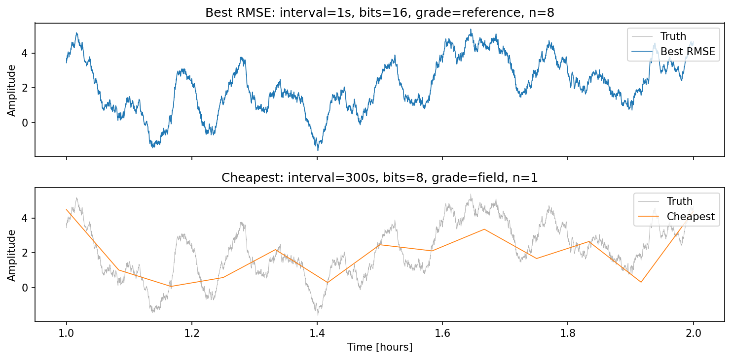
The best-RMSE design tracks every oscillation; the cheapest design misses the short-period modes entirely — exactly the trade-off the Pareto front quantifies.

Pareto front scatter matrix

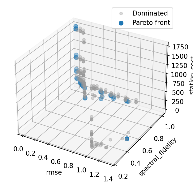
Each dot is one instrument configuration; highlighted points lie on the Pareto front. The RMSE–cost and fidelity–cost panels show the clear budget trade-off.

Parallel coordinates

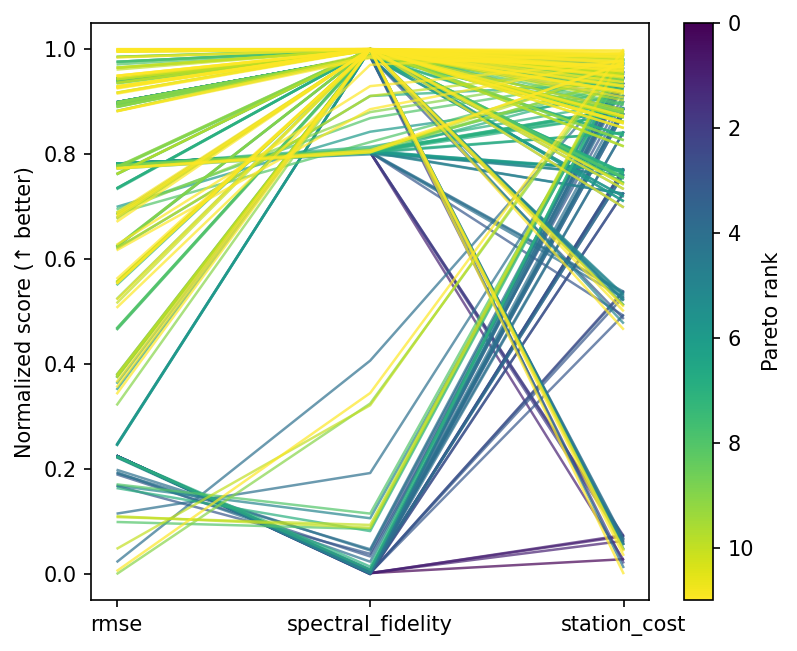
Every line is one design, coloured by Pareto membership. Front designs span from ultra-cheap to ultra-precise, with the mid-range configurations showing the sharpest cost-performance knee.

RMSE strip plot

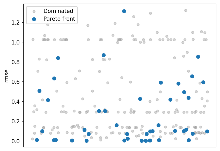
Scores split by Pareto membership. Most low-RMSE designs are on the front, while dominated designs cluster at higher error — confirming the front captures the best achievable accuracy at each cost level.

What to try next

• Use build_grid(factors, method="lhs", n_samples=60) for a Latin hypercube over continuous factor bounds.
• Wrap the sweep in a multi-phase Study — screen first with a coarse grid, then refine the promising region.
• Add an Annotation for power consumption or maintenance cost from an external costing sheet.
• Swap the brick-wall filter for a Butterworth via scipy.signal to study filter roll-off effects.