Hyperparameter Trade Study

This tutorial runs a multi-objective hyperparameter sweep over scikit-learn's GradientBoostingRegressor, balancing prediction accuracy against training cost and model complexity.

Run it yourself

The full runnable script is at examples/sklearn_study.py.

pip install scikit-learn
uv run python examples/sklearn_study.py

The problem

Machine learning practitioners routinely tune hyperparameters to minimize prediction error, but in production accuracy is not the only objective. A model that takes 10× longer to train or has 100× more parameters may not be worth the marginal RMSE improvement.

This example treats hyperparameter selection as a multi-objective design-of-experiments problem with three competing objectives:

Objective	Direction	What it measures
RMSE	minimize	Root mean squared error on a held-out test set
Training time	minimize	Wall-clock seconds to fit() the model
Complexity	minimize	Total number of leaf nodes across all trees

Why the objectives conflict

• More estimators → lower RMSE, but longer training and more leaves.
• Deeper trees → lower RMSE, but each tree has exponentially more leaves and takes longer to build.
• Higher learning rate → faster convergence with fewer trees, but risks overfitting if not paired with regularization.
• Lower subsample → implicit regularization (less overfitting), but noisier gradient estimates.

No single hyperparameter setting wins on all three objectives — the solutions lie on a Pareto front.

Dataset

We use scikit-learn's make_friedman1, a standard synthetic regression benchmark. The true function is:

\[y = 10\sin(\pi x_1 x_2) + 20(x_3 - 0.5)^2 + 10 x_4 + 5 x_5 + \varepsilon\]

where \(\varepsilon \sim \mathcal{N}(0, 1)\) and \(x_6, \dots, x_{10}\) are noise features. We generate 800 samples and hold out 25 % for testing:

X, y = make_friedman1(n_samples=800, noise=1.0, random_state=42)
X_train, X_test, y_train, y_test = train_test_split(
    X,
    y,
    test_size=0.25,
    random_state=42,
)

Simulator and scorer

In trade-study, every experiment needs a Simulator and a Scorer:

• The Simulator wraps model training. Its generate() method receives a hyperparameter config, fits a GradientBoostingRegressor, and returns the test-set ground truth plus predictions and metadata (training time, leaf count).
• The Scorer extracts the three objective values from each trial.

class GBSimulator:
    """Simulator that trains a GradientBoostingRegressor.

    The 'truth' is the test-set ground truth; 'observations' are the
    model's test-set predictions plus training metadata.
    """

    def generate(self, config: dict[str, Any]) -> tuple[Any, Any]:
        """Train a model and return predictions on the test set.

        Args:
            config: Hyperparameter dict with n_estimators, max_depth,
                learning_rate, and subsample.

        Returns:
            Tuple of (y_test array, observation dict with predictions,
            wall time, and number of leaves).
        """
        model = GradientBoostingRegressor(
            n_estimators=config["n_estimators"],
            max_depth=config["max_depth"],
            learning_rate=config["learning_rate"],
            subsample=config["subsample"],
            random_state=42,
        )
        t0 = time.perf_counter()
        model.fit(X_train, y_train)
        wall = time.perf_counter() - t0

        preds = model.predict(X_test)
        n_leaves = sum(tree[0].tree_.n_leaves for tree in model.estimators_)
        return y_test, {"predictions": preds, "wall": wall, "n_leaves": n_leaves}


class GBScorer:
    """Score GradientBoosting results for three objectives."""

    def score(
        self,
        truth: Any,
        observations: Any,
        config: dict[str, Any],
    ) -> dict[str, float]:
        """Compute RMSE, training time, and complexity.

        Args:
            truth: True target values (y_test).
            observations: Dict with predictions, wall time, n_leaves.
            config: Hyperparameter dict (unused).

        Returns:
            Scores for rmse, train_time, and complexity.
        """
        return {
            "rmse": root_mean_squared_error(truth, observations["predictions"]),
            "train_time": observations["wall"],
            "complexity": float(observations["n_leaves"]),
        }

Define observables and factors

Observables tell trade-study what you're measuring and which direction is better:

observables = [
    Observable("rmse", Direction.MINIMIZE),
    Observable("train_time", Direction.MINIMIZE),
    Observable("complexity", Direction.MINIMIZE),
]

Factors define the hyperparameter search space. We use discrete levels so a full factorial grid is tractable (\(4 \times 4 \times 4 \times 3 = 192\) combinations):

factors = [
    Factor("n_estimators", FactorType.DISCRETE, levels=[50, 100, 200, 400]),
    Factor("max_depth", FactorType.DISCRETE, levels=[2, 3, 4, 5]),
    Factor("learning_rate", FactorType.DISCRETE, levels=[0.01, 0.05, 0.1, 0.2]),
    Factor("subsample", FactorType.DISCRETE, levels=[0.6, 0.8, 1.0]),
]

Run the sweep

build_grid with method="full" generates every combination. run_grid evaluates them all and returns a ResultsTable:

    grid = build_grid(factors, method="full")
    print(f"Full factorial grid: {len(grid)} configurations")

    results = run_grid(
        world=GBSimulator(),
        scorer=GBScorer(),
        grid=grid,
        observables=observables,
    )

Hyperparameter landscape

Before looking at the Pareto front, it helps to see how RMSE varies across the two most influential hyperparameters. The heatmap below shows the best RMSE achieved at each (n_estimators, max_depth) combination, minimised over learning rate and subsample fraction:

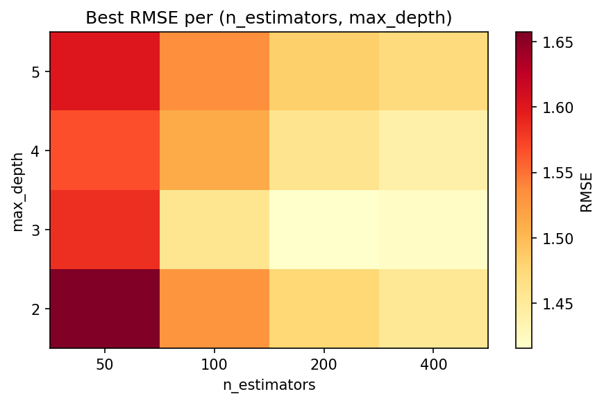
Deeper trees with more estimators push RMSE down, but at a cost in training time and model size — which is exactly the trade-off the Pareto front quantifies.

Inspect the Pareto front

extract_front identifies the subset of designs where no other design is better on all objectives simultaneously. Walking along the front reveals the fundamental trade-off: lower RMSE costs more training time and model complexity.

    # Pareto front
    front_idx = extract_front(
        results.scores,
        [o.direction for o in observables],
    )
    print(f"Pareto front: {len(front_idx)} / {len(grid)} designs\n")

    print(
        f"{'n_est':>6s}  {'depth':>5s}  {'lr':>6s}  {'sub':>5s}  "
        f"{'RMSE':>6s}  {'Time':>6s}  {'Leaves':>6s}"
    )
    print("-" * 52)
    for i in front_idx:
        cfg = results.configs[i]
        rmse, t, leaves = results.scores[i]
        print(
            f"{cfg['n_estimators']:6d}  {cfg['max_depth']:5d}  "
            f"{cfg['learning_rate']:6.2f}  {cfg['subsample']:5.1f}  "
            f"{rmse:6.3f}  {t:6.3f}  {leaves:6.0f}"
        )

    # Best RMSE on the front
    front_rmse = results.scores[front_idx, 0]
    best = front_idx[np.argmin(front_rmse)]
    print(f"\nLowest-RMSE Pareto design: {results.configs[best]}")
    print(
        f"  RMSE={results.scores[best, 0]:.4f}  "
        f"time={results.scores[best, 1]:.3f}s  "
        f"leaves={results.scores[best, 2]:.0f}"
    )

The Pareto front typically contains 10–15 designs out of 192. A practitioner can then choose based on their priorities — e.g. pick the lowest-RMSE design if accuracy is paramount, or the fastest design that still meets an RMSE threshold.

Pareto front scatter matrix

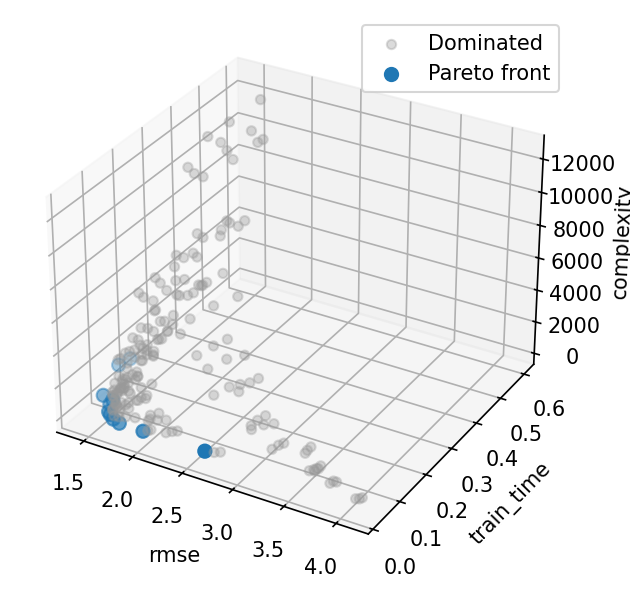
Each dot is one hyperparameter combination; highlighted points lie on the Pareto front. The off-diagonal panels expose pairwise trade-offs between RMSE, training time, and leaf count.

Parallel coordinates

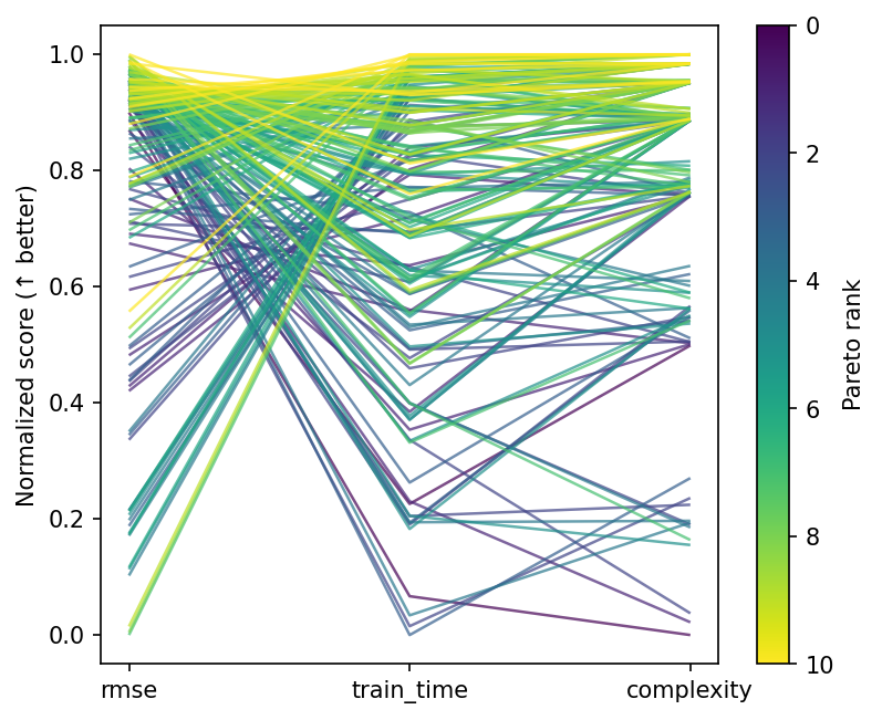
Every line is one design, coloured by Pareto membership. This view makes it easy to spot which hyperparameter ranges the front occupies.

RMSE strip plot

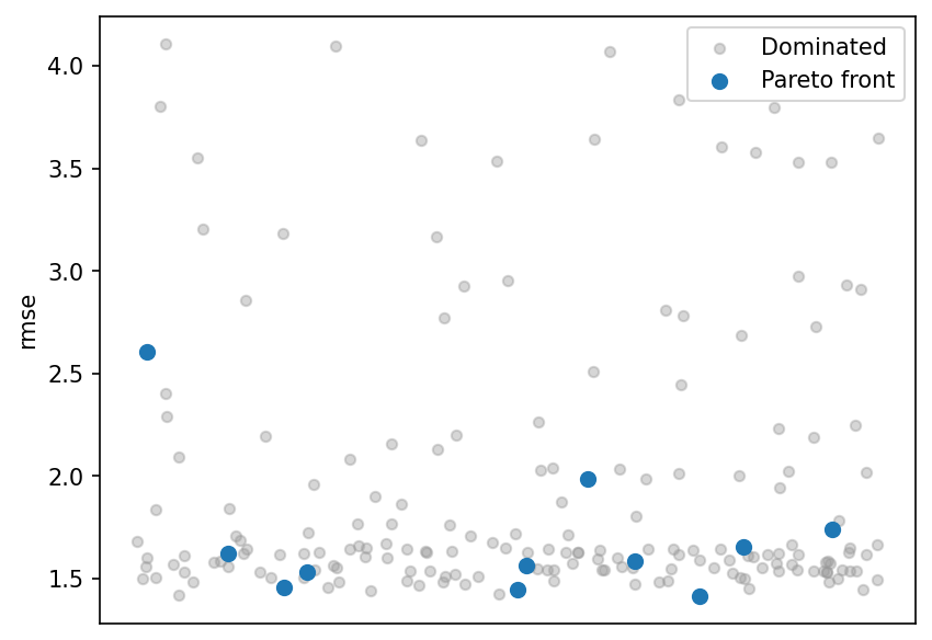
Scores for each design, split by whether it is on the Pareto front. Front members cluster at the low end of RMSE, confirming they are among the best predictive configurations.

What to try next

• Use build_grid(factors, method="lhs", n_samples=50) for a Latin hypercube design with continuous hyperparameters.
• Wrap the sweep in a Study with multiple phases — screen first, then refine the promising region.
• Add an Annotation for dollar cost (e.g., cloud compute pricing per second) to include cost as a non-simulated objective.
• Use save_results() / load_results() to persist results across sessions.